Solving a salary prediction problem with sklearn and pandas!
Problem Description
For a job search engine website, it’s helpful to suggest an approximate salary to job seekers for a given job post. Unfortunately, not all job postings include the salary. So the first task is to develop a salary prediction system. The goal is to provide estimated salaries for a new job posting.
Data Supplied
You are given three CSV (comma-separated) data files:
- train_features.csv: Each row represents metadata for an individual job posting.
The jobId column represents a unique identifier for the job posting. The remaining columns describe features of the job posting.
-
train_salaries.csv: Each row associates a
jobIdwith asalary. -
test_features.csv: Similar to train_features.csv, each row represents metadata for an individual job posting The first row of each file contains headers for the columns. Keep in mind that the metadata and salaries have been extracted by our aggregation and parsing systems. As such, it’s possible that the data is dirty (may contain errors).
The Task
We must build a model to predict the salaries for the job postings contained in test_features.csv. The output of the system should be a CSV file entitled test_salaries.csv where each row has the following format:
jobId,salary As a reference, the output should mirror the format of train_salaries.csv.
To judge the accuracy, we will compare salary predictions to a ground-truth using the root-mean-square error (RMSE).
How long did it take you to solve the problem?
It took me around 12 hours to solve this problem. It includes research, coding and generating output files (does not include time spent on writing this report).
What software language and libraries did you use to solve the problem? Why did you choose these languages/libraries?
-
Python - I used Python in this assignment since it is a multi-paradigm programming language. It supports object-oriented programming, structured programming, and functional programming patterns, among others. It has a large number of machine learning libraries build-around it that make processing and analyzing data simple and efficient.
-
Pandas - It is a powerful data manipulation and analysis library available for Python. I used it to effortlessly read csv data -
  import pandas as pd
  train_features = pd.read_csv("./DSciHomeworkAssignmentV2/train_features.csv")
  train_salaries = pd.read_csv("./DSciHomeworkAssignmentV2/train_salaries.csv")
I also used Pandas to perform a “join” between train_features.csv and train_salaries.csv on the key jobId -
data_train = pd.merge(train_features, train_salaries, on='jobId', how='outer')
and to extract relevant columns from the train data -
x_train = data_train[['companyId', 'jobType', 'degree', 'major', 'industry', 'yearsExperience', 'milesFromMetropolis']].values.reshape(-1, 7)
y_train = data_train['salary']
-
sklearn - I used it because of the large number of machine learning model implementations it provides
-
matplotlib - I used it to visualize a co-variance heat map
What steps did you take to prepare the data for the project? Was any cleaning necessary?
I did perform cleaning, a “join” and did a lot of feature engineering as explained below.
Step 1 - Read csv data and perform “join” -
Using Pandas, read CSV data and perform a “join” between train_features.csv and train_salaries.csv on the key jobId
Step 2 - Analyze data - We check for null values in the data
print(data_train.isnull().any())
and find that there are no null values as shown below -
| feature | Is null |
|---|---|
| jobId | False |
| companyId | False |
| jobType | False |
| degree | False |
| jobId | False |
| major | False |
| industry | False |
| yearsExperience | False |
| milesFromMetropolis | False |
| companyId | False |
| salary | False |
| companyId | False |
Then just to get an idea of what kind of value each feature takes, we print the unique values for each feature and see “NONE” being present in degree and major.
print(sorted(data_train['degree'].unique()))
print(sorted(data_train['major'].unique()))


['BACHELORS', 'DOCTORAL', 'HIGH_SCHOOL', 'MASTERS', 'NONE']}
{['BIOLOGY', 'BUSINESS', 'CHEMISTRY', 'COMPSCI', 'ENGINEERING', 'LITERATURE', 'MATH', 'NONE', 'PHYSICS']\end{lstlisting}
Hence, we establish that -
degreeandmajorhave null values present in the form of “NONE”degreeis ordinal. An ordinal feature is best described as a feature with natural, ordered categories and the distances between the categories is not known.jobType,major,industryandcompanyIdare nominal i.e., they do not have an order.jobIdis just an identifier used to map job features to salary.yearsExperienceandmilesFromMetropolisare numerical features i.e., they are continuous numeric values.
Step 3 - Find significance of features -
To identify the significance of features, I performed the following steps -
- Created a list
columnscontaining names of every column in thedata_train - Drop
jobIdfrom thecolumnssincejobIdis just an identifier used to map job features to salary (line 6). -
Generate the co-variance matrix for the features and visualize it as a heat map (lines 8 - 12)
  import seaborn as sns
  import matplotlib.pyplot as plt
  def analyze_feature_correlation(self):
      columns = list(data_train.columns.values).remove("jobId")
      correlation_map = np.corrcoef(data_train[columns].values.T)
      sns.set(font_scale=1.0)
      heatmap = sns.heatmap(correlation_map, cbar=True, annot=True, square=True, fmt='.2f', yticklabels=columns, xticklabels=columns)
  plt.show()
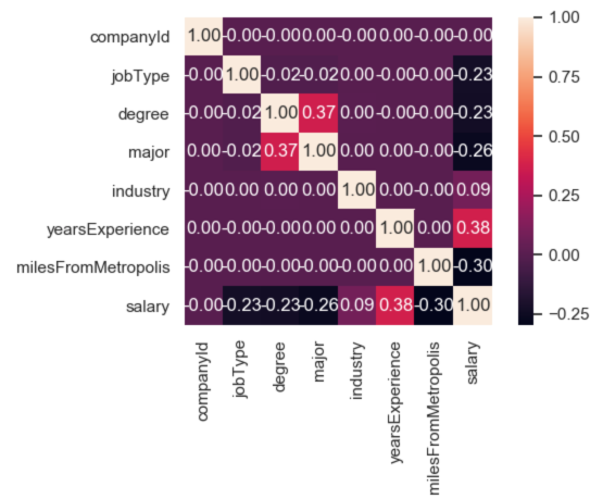
Step 4 - Analyzing covariance matrix -
To interpret the meaning of the covariance matrix, we can use the definition of covariance which says that it is a measure of the joint variability of two random variables. If the greater values of one variable mainly correspond with the greater values of the other variable, and the same holds for the lesser values, (i.e., the variables tend to show similar behavior), the covariance is positive. In the opposite case, when the greater values of one variable mainly correspond to the lesser values of the other, (i.e., the variables tend to show opposite behavior), the covariance is negative.
I was able to draw the following inferences from the above shown graphic -
-
yearsExperiencehas the highest normalized covariance magnitude (0.38) in the matrix. This makesyearsExperiencethe feature which has the greatest impact onsalary. The fact that the sign of it’s conavirance is positive, means that greateryearsExperiencewill lead to greatersalary. -
companyIdhas the the lowest normalized covariance magnitude (0.00) in the matrix. This makescompanyIdthe feature which has the least impact onsalary. -
milesFromMetropolishas a large negative normalized covariance magnitude (-0.30). The fact that the sign of it’s conavirance is negative, means that greatermilesFromMetropoliswill lead to lesssalary.
Step 5 - Feature engineering (Important) -
Based on the facts and analysis presented above, I engineered my features in the following manner -
- Drop
jobIdfrom the dataframe sincejobIdis just an identifier used to map job features to salary - Drop
companyIdfrom the dataframe sincecompanyIdhas zero co-variance value -
Impute (fill up) the null values in
degreeandmajorwithSimpleImputerby inserting the most frequent label in each column to null cells.from sklearn.impute import SimpleImputer imputer = SimpleImputer(missing_values=np.nan, strategy="most_frequent") imputer = imputer.fit(data_train.loc[:int(row / 4), 'degree':'major']) data_train.loc[:, 'degree':'major'] = imputer.transform(data_train.loc[:, 'degree':'major']) -
Encode
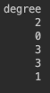
degreewith the OrdinalEncoder class. To make sure that order is respected i.e., DOCTORAL is given highest value and HIGH_SCHOOL least, we pass an ordered list of unique values for the feature to the categories parameter.from sklearn.preprocessing import OrdinalEncoder self.ordinal_encoder = OrdinalEncoder() cat = pd.Categorical(data_train.degree, categories=['HIGH_SCHOOL', 'BACHELORS', 'MASTERS', 'DOCTORAL'], ordered=True) labels, unique = pd.factorize(cat, sort=True) data_train.degree = labels data_train.degree = self.ordinal_encoder.fit_transform(data_train.degree.values.reshape(-1, 1))
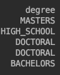 becomes
-
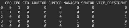
Encode nominal features (
jobType,majorandindustry) with one-hot-encoding where each categorical feature with n categories is transformed into n binary features.from sklearn.preprocessing import OneHotEncoder self.onehot_encoder = OneHotEncoder(dtype=np.int, sparse=True) nominals = pd.DataFrame(self.onehot_encoder.fit_transform(data_train[['jobType', 'major', 'industry']]).toarray(), columns=[nominal_cols])
For example,

becomes
-
Discretization, also known as quantization or binning, divides a continuous feature into a pre-specified number of categories (bins), and thus makes the data discrete. So, we can use discretization to make
yearsExperienceandmilesFromMetropolisdiscrete.An important point to note here is that
milesFromMetropolishas a large negative covariance with salary. So we need to make sure large values ofmilesFromMetropolis(for e.x., 83) are assigned small values of bin (for e.x., 3.0). To make this change, we make allmilesFromMetropolisnegative so that their bin order would be reversed. ForyearsExperience, we will use the ordinal ordering since largeyearsExperiencemeans largesalary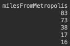 becomes
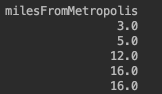
  from sklearn.preprocessing import KBinsDiscretizer

  nominals['milesFromMetropolis'] = nominals['milesFromMetropolis'].apply(lambda x: -x)

  disc = KBinsDiscretizer(n_bins=8, encode='ordinal', strategy='quantile')
  disc.fit(nominals.loc[:, 'yearsExperience'])
  nominals.loc[:, 'yearsExperience'] = disc.transform(nominals.loc[:, 'yearsExperience'])

  disc = KBinsDiscretizer(n_bins=20, encode='ordinal', strategy='quantile')
  disc.fit(nominals.loc[:, 'milesFromMetropolis'])
  nominals.loc[:, 'milesFromMetropolis'] = disc.transform(nominals.loc[:, 'milesFromMetropolis'])
a)What machine learning method did you apply?
I applied sklearn.RandomForestRegressor method
b) Why did you choose this method?
I selected RandomForestRegressor because it uses bootstrap aggregating or bagging, to decision tree learners. Bagging repeatedly selects a random sample with replacement from the training set and fits trees to these samples. Since we are using multiple learning algorithms, it has the effect of producing better predictive results that could have been obtained from any of the constituent learning algorithms alone.
Another reason why Random Forests lead to better model performance is that they decrease the variance (reducing over-fitting) of the model, without increasing the bias (keeping under-fitting in check). In other words, the predictions of a single tree are highly sensitive to noise in its training set, the average of many trees is not, as long as the trees are not correlated i.e., they are trained on different training sets.
I compared the cross-validation RMSE values for various models as shown below. Even though PolynomialLinearRegression performs better than RandomForestRegressor, the accuracy of RandomForestRegressor can be increased by increasing the number of n_estimators.
def check_algorithm_performance(self):
    X, Y = self.get_train_data()
    X_train, X_test, Y_train, Y_test = train_test_split(X, Y, test_size=0.20, random_state=42)

    pipelines = list()
    pipelines.append(('LinearRegression', Pipeline([('LR', LinearRegression())])))
    pipelines.append(('PolynomialLinearRegression', Pipeline([('PLR', PolynomialFeatures(degree=2)), ('linear', linear_model.LinearRegression(fit_intercept=False))])))
    pipelines.append(('RandomForestRegressor', Pipeline([('RF', RandomForestRegressor(n_estimators=10, n_jobs=6, max_depth=20))])))

    results = []
    names = []
    for name, model in pipelines:
        kfold = KFold(n_splits=5, random_state=21)
        cv_results = np.sqrt(-1 * cross_val_score(model, X_train, Y_train, cv=kfold, scoring='neg_mean_squared_error'))
        results.append(cv_results)
        names.append(name)
        msg = "%s: %f" % (name, cv_results.mean())
        print(msg)
As shown below, RandomForestRegressor produced the lowest RMSE on cross validation data.
| Regression model | Cross validation RMSE |
|---|---|
| LinearRegression | 20.336951 |
| PolynomialLinearRegression | 19.609648 |
| RandomForestRegressor | 20.284646 |
Describe how the machine learning method that you chose works.
-
Regression Random forests are an ensemble learning method for regression that operate by constructing a number of decision trees at training time and outputting the mean prediction of the individual trees.
-
General Decision Tree step - A decision tree can be “learned” by splitting the data set into subsets based on an attribute value test. This process is repeated on each derived subset in a recursive manner. The recursion is completed when the subset at a node has all the same value of the target variable, or when splitting no longer adds value to the predictions or when a user specified tree depth is reached. This process of top-down induction of decision trees is an example of a greedy algorithm.
Bagging- Given a training set X = x1 , …, xn with responses Y = y1, …, yn, bagging repeatedly (B times) selects a random sample with replacement of the training set and fits trees to these samples:
For b = 1, …, B:
  * Sample, with replacement, n training examples from X, Y; call these X<sub>b</sub>, Y<sub>b</sub>.
  * Train a classification or regression tree f<sub>b</sub> on X<sub>b</sub>, Y<sub>b</sub>.
After training, predictions for unseen samples can be made by averaging the predictions from all the individual regression trees.
- Random forest step - Random forests use a modified tree learning algorithm that selects, at each candidate split in the learning process, a random subset of the features. The reason for doing this is the correlation of the trees in an ordinary bootstrap sample: if one or a few features are very strong predictors for the response variable (target output), these features will be selected in many of the B trees, causing them to become correlated.
How did you train your model? During training, what issues concerned you?
- I trained my model by performing the following steps -
- Get train features in X and train salaries in Y
- Create a RandomForestRegressor model
-
Train/fit the model on X and Y
  def predict(self):
      X, Y = self.get_train_data()
      model = RandomForestRegressor(n_estimators=5, random_state=0)
      model.fit(X, Y)
During training, the issues that concerned me were -
- Training time of my model
- Value of parameters (such as n_estimators etc.) that would produce the best model
a) Estimate the RMSE that your model will achieve on the test data-set.
RMSE that my model will achieve on test data-set would be around 20.284646
b) How did you create this estimate?
To estimate the RMSE that I would get on test data-set I created my own pseudo-test data-set by dividing the labeled train data-set in 80:20 ratio. I used the 80% data as train and other 20% as test to calculate RMSE.
X, Y = self.get_train_data()
X_train, X_test, Y_train, Y_test = train_test_split(X, Y, test_size=0.20, random_state=42)
It can be safely assumed that given some other unseen data, my model will achieve RMSE comparable to the one I calculated above.
What metrics, other than RMSE, would be useful for assessing the accuracy of salary estimates? Why?
-
Median absolute error (MAE) is calculated by taking the median of all absolute differences between the target and the prediction. Particularly interesting because it is robust to outliers.
-
Mean absolute percentage error(MAPE) is the percentage equivalent of MAE. The equation looks just like that of MAE, but with adjustments to convert everything into percentages. Just as MAE is the average magnitude of error produced by your model, the MAPE is how far the model’s predictions are off from their corresponding outputs on average. Like MAE, MAPE also has a clear interpretation since percentages are easier for people to conceptualize. Both MAPE and MAE are robust to the effects of outliers thanks to the use of absolute value.